[1]:
import matplotlib as mpl
import matplotlib.pyplot as plt
import numpy as np

mpl.rcParams.update(
    {
        "text.usetex": False,
        "axes.labelsize": 18,
        "xtick.labelsize": 15,
        "ytick.labelsize": 15,
        "figure.constrained_layout.wspace": 0,
        "figure.constrained_layout.hspace": 0,
        "figure.constrained_layout.h_pad": 0,
        "figure.constrained_layout.w_pad": 0,
        "axes.linewidth": 1.3,
    }
)

import jax
import jax.numpy as jnp

# you should always set this
jax.config.update("jax_enable_x64", True)
Matplotlib is building the font cache; this may take a moment.
Damped Random Walk (DRW)#
The Gaussian Process (GP) kernel corresponding to a Damped Random Walk (DRW) process is
where \(|\Delta t|\) denotes the time separation between two observations. The parameter \(\ell\) represents the correlation length scale of the process, while \(\sigma^2\) is the asymptotic variance of the GP. In EzTaoX, this kernel is implemented via the kernels.quasisep.Exp class.
Note
In the astronomy literature, a DRW process is commonly parameterized by a damping timescale \(\tau_{\rm DRW}\) and a root-mean-square (RMS) variability amplitude \(\sigma_{\rm DRW}\). The correspondence with the Exp kernel parameters is:
\(\tau_{\rm DRW} = \ell\) (the correlation length scale),
\(\sigma_{\rm DRW} = \sigma\) (the standard deviation, i.e., square root of the asymptotic variance).
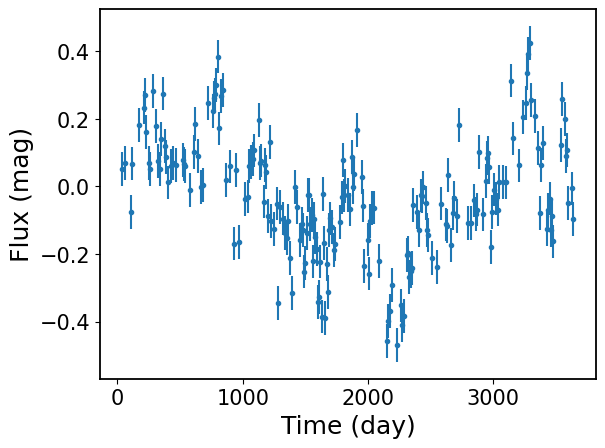
1. Light Curve Simulation#
We use UniVarSim to simulate DRW light curves
[2]:
from eztaox.kernels.quasisep import Exp
from eztaox.simulator import UniVarSim
from eztaox.ts_utils import add_noise
[3]:
# Simulated DRW parameters
drw_scale, drw_sigma = 100.0, 0.15
sim_params = {"log_kernel_param": jnp.log(jnp.asarray([drw_scale, drw_sigma]))}


# initiate univariate (i.e., single-band) simulator
min_dt, max_dt = 10, 3650.0
s = UniVarSim(Exp(*sim_params["log_kernel_param"]), min_dt, max_dt, sim_params)

# simulate light curve, add noise
sim_t, sim_y = s.random(200, jax.random.PRNGKey(0), jax.random.PRNGKey(1))
sim_yerr = jnp.ones_like(sim_t) * 0.05
sim_y_noisy = add_noise(sim_y, sim_yerr, jax.random.PRNGKey(2))
[4]:
plt.errorbar(sim_t, sim_y_noisy, sim_yerr, fmt=".")

plt.xlabel("Time (day)")
plt.ylabel("Flux (mag)")
[4]:
Text(0, 0.5, 'Flux (mag)')
2. Fitting#
Here, we demonstrate how to use the UniVarModel for fitting single-band light curves.
[5]:
import numpyro
import numpyro.distributions as dist
from eztaox.fitter import random_search
from eztaox.models import UniVarModel
from numpyro.handlers import seed as numpyro_seed
2.1 Initialize Light Curve Model#
[6]:
# whether assuming the input light curve have mean of zero
zero_mean = False

# initialize a GP kernel, note the initial parameters are not used in the fitting
k = Exp(scale=100.0, sigma=1.0)
m = UniVarModel(sim_t, sim_y_noisy, sim_yerr, k, zero_mean=zero_mean)
m
[6]:
UniVarModel(
  X=(f64[200], i64[200]),
  y=f64[200],
  diag=f64[200],
  base_kernel_def=<jax._src.util.HashablePartial object at 0x7cd8dcb62e90>,
  multiband_kernel=<class 'eztaox.kernels.quasisep.MultibandLowRank'>,
  t_in_bands=[f64[200]],
  concat_inds_in_bands=i64[200],
  n_band=1,
  mean_func=None,
  amp_scale_func=None,
  lag_func=None,
  zero_mean=False,
  has_jitter=False,
  has_lag=False
)
2.2 Define Init Sampler#
[7]:
def init_sampler():
    # GP kernel param
    log_drw_scale = numpyro.sample(
        "log_drw_scale", dist.Uniform(jnp.log(0.01), jnp.log(1000))
    )
    log_drw_sigma = numpyro.sample(
        "log_drw_sigma", dist.Uniform(jnp.log(0.01), jnp.log(10))
    )
    log_kernel_param = jnp.stack([log_drw_scale, log_drw_sigma])
    numpyro.deterministic("log_kernel_param", log_kernel_param)

    # mean
    mean = numpyro.sample("mean", dist.Uniform(low=-0.2, high=0.2))

    sample_params = {"log_kernel_param": log_kernel_param, "mean": mean}
    return sample_params
[8]:
# generate a random initial guess
sample_key = jax.random.PRNGKey(1)
prior_sample = numpyro_seed(init_sampler, rng_seed=sample_key)()
prior_sample
[8]:
{'log_kernel_param': Array([-2.19138685,  0.3506587 ], dtype=float64),
 'mean': Array(-0.06222013, dtype=float64)}
2.3 MLE Fitting#
[9]:
%%time
model = m
sampler = init_sampler
fit_key = jax.random.PRNGKey(1)
n_sample = 10_000

n_best = 10  # it seems like this number needs to be high

bestP, ll = random_search(model, init_sampler, fit_key, n_sample, n_best)
bestP
CPU times: user 1.79 s, sys: 54.3 ms, total: 1.84 s
Wall time: 1.82 s
[9]:
{'log_kernel_param': Array([ 4.65322136, -1.80981286], dtype=float64),
 'mean': Array(-0.01944095, dtype=float64)}
[10]:
print("True DRW Params (in natual log):")
print(np.log(np.hstack([drw_scale, drw_sigma])))
print("MLE DHO Params (in natual log):")
print(bestP["log_kernel_param"])
True DRW Params (in natual log):
[ 4.60517019 -1.89711998]
MLE DHO Params (in natual log):
[ 4.65322136 -1.80981286]
3. MCMC#
[11]:
import arviz as az
from numpyro.infer import MCMC, NUTS, init_to_median
/home/docs/checkouts/readthedocs.org/user_builds/eztaox/envs/stable/lib/python3.11/site-packages/arviz/__init__.py:50: FutureWarning:
ArviZ is undergoing a major refactor to improve flexibility and extensibility while maintaining a user-friendly interface.
Some upcoming changes may be backward incompatible.
For details and migration guidance, visit: https://python.arviz.org/en/latest/user_guide/migration_guide.html
  warn(
[12]:
def numpyro_model(m):
    sample_params = init_sampler()
    m.sample(sample_params)
[13]:
%%time
zero_mean = False
k = Exp(scale=100.0, sigma=1.0)  # init params for k are not used
m = UniVarModel(sim_t, sim_y_noisy, sim_yerr, k, zero_mean=zero_mean)

nuts_kernel = NUTS(
    numpyro_model,
    dense_mass=True,
    target_accept_prob=0.9,
    init_strategy=init_to_median,
)

mcmc = MCMC(
    nuts_kernel,
    num_warmup=1000,
    num_samples=5000,
    num_chains=1,
    # progress_bar=False,
)

mcmc_seed = 0
mcmc.run(jax.random.PRNGKey(mcmc_seed), m)

data = az.from_numpyro(mcmc)
mcmc.print_summary()
sample: 100%|██████████| 6000/6000 [00:02<00:00, 2457.46it/s, 7 steps of size 4.48e-01. acc. prob=0.95]
                     mean       std    median      5.0%     95.0%     n_eff     r_hat
  log_drw_scale      4.89      0.39      4.84      4.24      5.45   1275.53      1.00
  log_drw_sigma     -1.71      0.18     -1.74     -1.99     -1.46   1334.72      1.00
           mean     -0.02      0.05     -0.02     -0.10      0.07   2881.55      1.00

Number of divergences: 0
CPU times: user 4.67 s, sys: 178 ms, total: 4.85 s
Wall time: 4.82 s
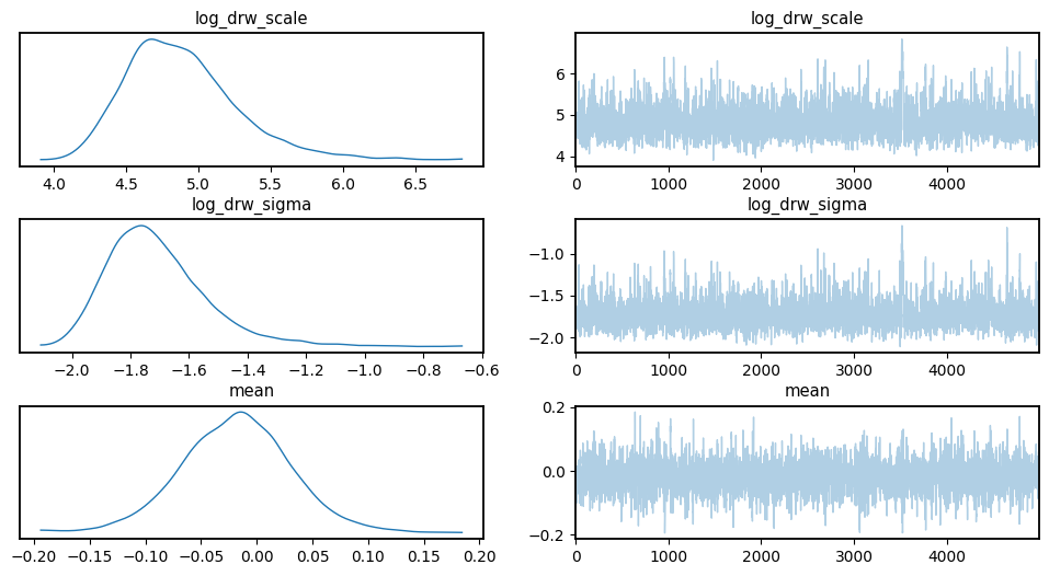
Visualize Chains, Posterior Distributions#
[14]:
import warnings

warnings.filterwarnings("ignore", category=RuntimeWarning)
[15]:
az.plot_trace(
    data,
    var_names=["log_drw_scale", "log_drw_sigma", "mean"],
)
plt.subplots_adjust(hspace=0.4)
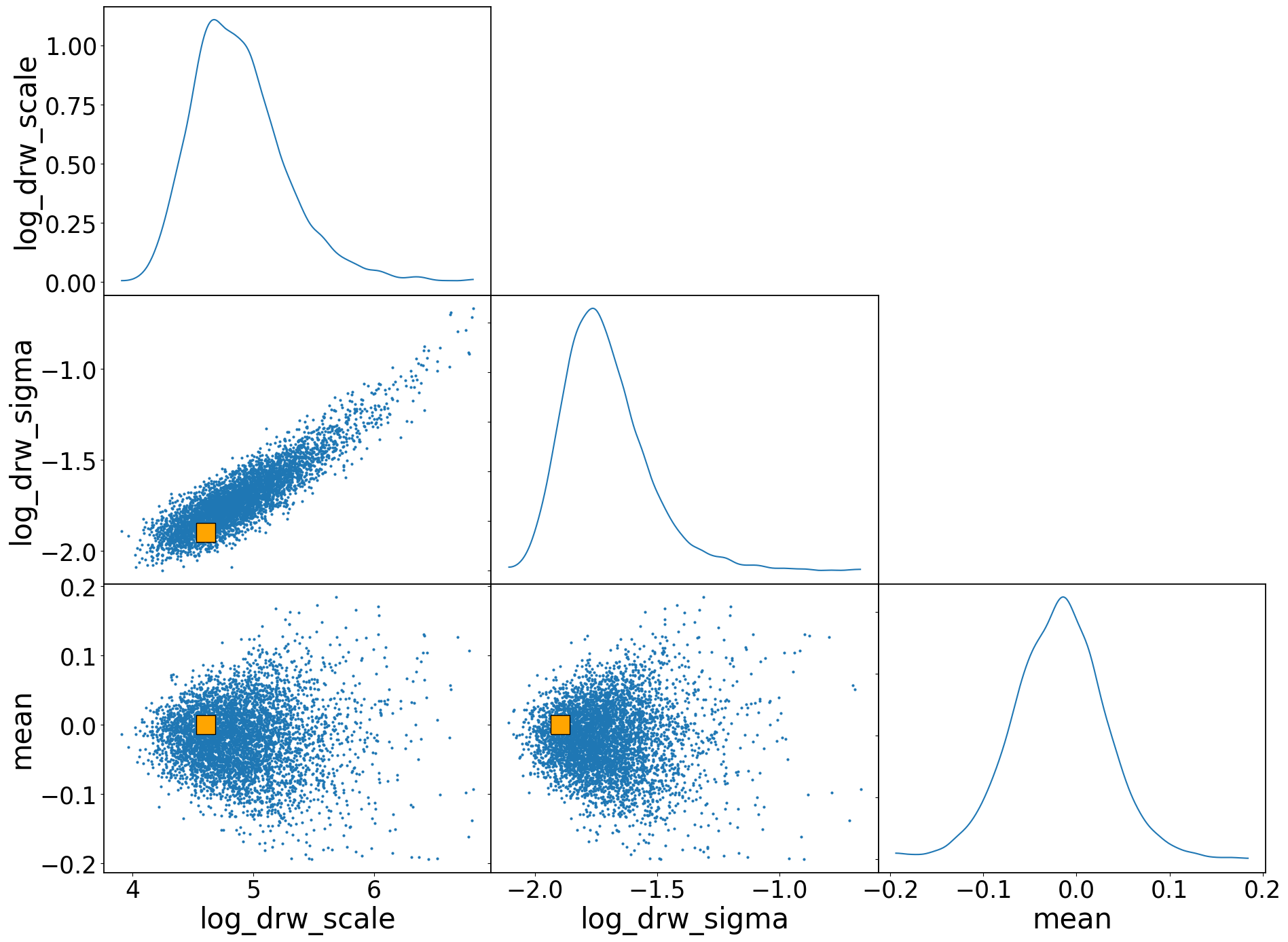
[16]:
az.plot_pair(
    data,
    var_names=["log_drw_scale", "log_drw_sigma", "mean"],
    reference_values={
        "log_drw_scale": np.log(drw_scale),
        "log_drw_sigma": np.log(drw_sigma),
        "mean": 0.0,
    },
    reference_values_kwargs={"color": "orange", "markersize": 20, "marker": "s"},
    kind="scatter",
    marginals=True,
    textsize=25,
)
plt.subplots_adjust(hspace=0.0, wspace=0.0)
4. Second-order Statistics#
[17]:
from eztaox.kernel_stat2 import gpStat2

ts = np.logspace(0, 4)
fs = np.logspace(-4, 0)
[18]:
# get MCMC samples
flatPost = data.posterior.stack(sample=["chain", "draw"])
log_drw_draws = flatPost["log_kernel_param"].values.T
[19]:
# create second-order stat object
drw_k = Exp(scale=drw_scale, sigma=drw_sigma)
gpStat2_drw = gpStat2(drw_k)
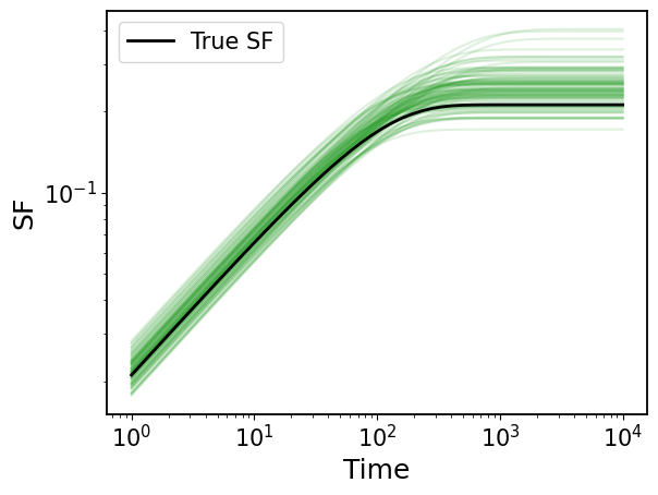
4.1 Structure Function#
[20]:
# compute sf for MCMC draws
mcmc_sf = jax.vmap(gpStat2_drw.sf, in_axes=(None, 0))(ts, jnp.exp(log_drw_draws))
[21]:
## plot
# ture SF
plt.loglog(ts, gpStat2_drw.sf(ts), c="k", label="True SF", zorder=100, lw=2)
plt.legend(fontsize=15)
# MCMC SFs
for sf in mcmc_sf[::50]:
    plt.loglog(ts, sf, c="tab:green", alpha=0.15)

plt.xlabel("Time")
plt.ylabel("SF")
[21]:
Text(0, 0.5, 'SF')
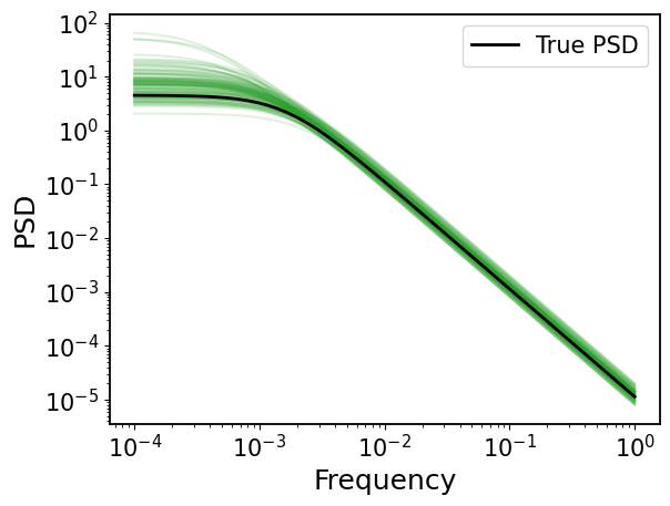
4.1 Power Spectral Density (PSD)#
[22]:
# compute sf for MCMC draws
mcmc_psd = jax.vmap(gpStat2_drw.psd, in_axes=(None, 0))(fs, jnp.exp(log_drw_draws))
[23]:
## plot
# ture PSD
plt.loglog(fs, gpStat2_drw.psd(fs), c="k", label="True PSD", zorder=100, lw=2)
plt.legend(fontsize=15)

# MCMC PSDs
for psd in mcmc_psd[::50]:
    plt.loglog(fs, psd, c="tab:green", alpha=0.15)

plt.xlabel("Frequency")
plt.ylabel("PSD")
[23]:
Text(0, 0.5, 'PSD')