[1]:

import matplotlib as mpl
import matplotlib.pyplot as plt
import numpy as np
import warnings

warnings.filterwarnings("ignore", category=RuntimeWarning)

mpl.rcParams.update(
    {
        "text.usetex": False,
        "axes.labelsize": 18,
        "xtick.labelsize": 15,
        "ytick.labelsize": 15,
        "figure.constrained_layout.wspace": 0,
        "figure.constrained_layout.hspace": 0,
        "figure.constrained_layout.h_pad": 0,
        "figure.constrained_layout.w_pad": 0,
        "axes.linewidth": 1.3,
    }
)

import jax
import jax.numpy as jnp

# you should always set this
jax.config.update("jax_enable_x64", True)

Damped Random Walk (DRW)#

The Gaussian Process (GP) kernel corresponding to a Damped Random Walk (DRW) process is

\[k(|\Delta t|) = \sigma^2 \exp \left(-\frac{|\Delta t|}{\ell}\right),\]

where \(|\Delta t|\) denotes the time separation between two observations. The parameter \(\ell\) represents the correlation length scale of the process, while \(\sigma^2\) is the asymptotic variance of the GP. In EzTaoX, this kernel is implemented via the kernels.quasisep.Exp class.

Note

In the astronomy literature, a DRW process is commonly parameterized by a damping timescale \(\tau_{\rm DRW}\) and a root-mean-square (RMS) variability amplitude \(\sigma_{\rm DRW}\). The correspondence with the Exp kernel parameters is:

\(\tau_{\rm DRW} = \ell\) (the correlation length scale),
\(\sigma_{\rm DRW} = \sigma\) (the standard deviation, i.e., square root of the asymptotic variance).

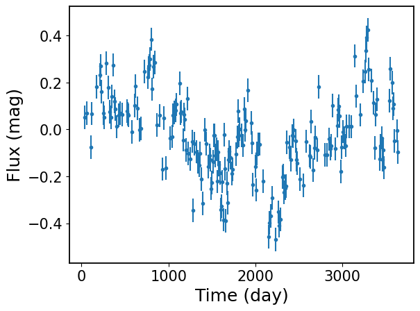
1. Light Curve Simulation#

We use UniVarSim to simulate DRW light curves

[2]:

from eztaox.kernels.quasisep import Exp
from eztaox.simulator import UniVarSim
from eztaox.ts_utils import add_noise

[3]:

# Simulated DRW parameters
drw_scale, drw_sigma = 100.0, 0.15
sim_params = {"log_kernel_param": jnp.log(jnp.asarray([drw_scale, drw_sigma]))}


# initiate univariate (i.e., single-band) simulator
min_dt, max_dt = 10, 3650.0
s = UniVarSim(Exp(*sim_params["log_kernel_param"]), min_dt, max_dt, sim_params)

# simulate light curve, add noise
sim_t, sim_y = s.random(200, jax.random.PRNGKey(0), jax.random.PRNGKey(1))
sim_yerr = jnp.ones_like(sim_t) * 0.05
sim_y_noisy = add_noise(sim_y, sim_yerr, jax.random.PRNGKey(2))

[4]:

plt.errorbar(sim_t, sim_y_noisy, sim_yerr, fmt=".")
plt.xlabel("Time (day)")
plt.ylabel("Flux (mag)")

[4]:

Text(0, 0.5, 'Flux (mag)')

2. Light Curve Fitting#

Here, we demonstrate how to use the UniVarModel to fit single-band light curves.

[5]:

import numpyro
import numpyro.distributions as dist
from eztaox.fitter import random_search
from eztaox.models import UniVarModel
from numpyro.handlers import seed as numpyro_seed

2.1 Initialize Light Curve Model#

[6]:

# whether assuming the input light curve have mean of zero
zero_mean = False

# initialize a GP kernel, note the initial parameters are not used in the fitting
k = Exp(scale=100.0, sigma=1.0)
m = UniVarModel(sim_t, sim_y_noisy, sim_yerr, k, zero_mean=zero_mean)
m

[6]:

UniVarModel(
  X=(f64[200], i64[200]),
  y=f64[200],
  diag=f64[200],
  base_kernel_def=<jax._src.util.HashablePartial object at 0x79be21817510>,
  multiband_kernel=<class 'eztaox.kernels.quasisep.MultibandLowRank'>,
  t_in_bands=[f64[200]],
  concat_inds_in_bands=i64[200],
  n_band=1,
  mean_func=None,
  amp_scale_func=None,
  lag_func=None,
  zero_mean=False,
  has_jitter=False,
  has_lag=False
)

2.2 Define Init Sampler#

The init_sampler defines a prior distribution from which random samples are drawn for likelihood evaluation. The distribution for a parameter can take any shape, as long as it has a numpyro implementation. A list of numpyro distributions can be found here.

Model parameters:

log_drw_scale: The natual log of the \(\ell\) parameter of the Exp kernel.
log_drw_sigma: The natual log of the \(\sigma\) of the Exp kernel.
log_kernel_param: The parameters of the latent GP process.
mean: The mean of the light curve in each band, with a size M.

[7]:

def init_sampler():
    # GP kernel param
    log_drw_scale = numpyro.sample(
        "log_drw_scale", dist.Uniform(jnp.log(0.01), jnp.log(1000))
    )
    log_drw_sigma = numpyro.sample(
        "log_drw_sigma", dist.Uniform(jnp.log(0.01), jnp.log(10))
    )
    log_kernel_param = jnp.stack([log_drw_scale, log_drw_sigma])
    numpyro.deterministic("log_kernel_param", log_kernel_param)

    # mean
    mean = numpyro.sample("mean", dist.Uniform(low=-0.2, high=0.2))

    sample_params = {"log_kernel_param": log_kernel_param, "mean": mean}
    return sample_params

[8]:

# generate a random initial guess
sample_key = jax.random.PRNGKey(1)
prior_sample = numpyro_seed(init_sampler, rng_seed=sample_key)()
prior_sample

[8]:

{'log_kernel_param': Array([-2.19138685,  0.3506587 ], dtype=float64),
 'mean': Array(-0.06222013, dtype=float64)}

2.3 MLE Fitting#

To find the best-fit parameters, one can start at a random point in the parameter space and optimize the likelihood function until it stops changing. The likelihood for any given set of parameters can be evaluated by calling UniVarModel.log_prob(params). However, this approach can often stuck in local minima. EzTaoX provides a fit function (random_search) to alleviate this issue (to some level). The random_search function first does a random search (i.e., evaluate the likelihood at a large number of randomly chosen positions in the parameter space) and then select a few (defaults to five) positions with the highest likelihood to proceed with additional local optimization (e.g., using the Adam optimizer).

The random_search function takes the following arguments:

model: an instance of UniVarModel
init_sampler: a custom function (you need to provide) for generating random samples for the random search step.
prng_key: a JAX random number generator key.
n_sample: number of random samples to draw.
n_best: number of best samples to keep for continued optimization.
batch_size: The number of likelihoods to evaluate each time. Defaults to 1000, for simpler models (and if you have enough memory), you can set this to n_sample.

[9]:

%%time
model = m
sampler = init_sampler
fit_key = jax.random.PRNGKey(1)
n_sample = 10_000
n_best = 10  # it seems like this number needs to be high

# run random search to find the best parameters
bestP, ll = random_search(model, init_sampler, fit_key, n_sample, n_best)

print("True DRW Params (in natual log):")
print(np.log(np.hstack([drw_scale, drw_sigma])))
print("MLE DHO Params (in natual log):")
print(bestP["log_kernel_param"])
print("-" * 50)

True DRW Params (in natual log):
[ 4.60517019 -1.89711998]
MLE DHO Params (in natual log):
[ 4.65322136 -1.80981286]
--------------------------------------------------
CPU times: user 2.26 s, sys: 82 ms, total: 2.34 s
Wall time: 2.29 s

3. MCMC#

MCMC sampling is carried out using the numpyro package, which is native to JAX. In this example, I will use the NUTS algorithm; however, there is a large collection of sampling algorithms that you can pick from (see here). In addition, you can freely specify more flexible (no longer just flat!!) prior distributions for each parameter in the light curve model.

[10]:

import arviz as az
from numpyro.infer import MCMC, NUTS, init_to_median

/home/docs/checkouts/readthedocs.org/user_builds/eztaox/envs/latest/lib/python3.11/site-packages/arviz/__init__.py:50: FutureWarning:
ArviZ is undergoing a major refactor to improve flexibility and extensibility while maintaining a user-friendly interface.
Some upcoming changes may be backward incompatible.
For details and migration guidance, visit: https://python.arviz.org/en/latest/user_guide/migration_guide.html
  warn(

3.1 Define `Numpyro` Model#

[11]:

def numpyro_model(m):
    # GP kernel param
    log_drw_scale = numpyro.sample(
        "log_drw_scale", dist.Uniform(jnp.log(0.01), jnp.log(1000))
    )
    log_drw_sigma = numpyro.sample(
        "log_drw_sigma", dist.Uniform(jnp.log(0.01), jnp.log(10))
    )
    log_kernel_param = jnp.stack([log_drw_scale, log_drw_sigma])
    numpyro.deterministic("log_kernel_param", log_kernel_param)

    # mean
    mean = numpyro.sample("mean", dist.Uniform(low=-0.2, high=0.2))

    sample_params = {"log_kernel_param": log_kernel_param, "mean": mean}
    m.sample(sample_params)

THe prior distribution definition shares the same syntax as the init_sampler, thus, one can reuse the init_sampler in the numpyro_model if the prior distribution doesn’t change. For example,

def numpyro_model(m):
    sample_params = init_sampler()
    m.sample(sample_params)

[12]:

%%time
zero_mean = False
k = Exp(scale=100.0, sigma=1.0)  # init params for k are not used
m = UniVarModel(sim_t, sim_y_noisy, sim_yerr, k, zero_mean=zero_mean)

nuts_kernel = NUTS(
    numpyro_model,
    dense_mass=True,
    target_accept_prob=0.9,
    init_strategy=init_to_median,
)

mcmc = MCMC(
    nuts_kernel,
    num_warmup=1000,
    num_samples=5000,
    num_chains=1,
    # progress_bar=False,
)

mcmc_seed = 0
mcmc.run(jax.random.PRNGKey(mcmc_seed), m)

data = az.from_numpyro(mcmc)
mcmc.print_summary()

sample: 100%|██████████| 6000/6000 [00:03<00:00, 1808.19it/s, 15 steps of size 4.06e-01. acc. prob=0.95]


                     mean       std    median      5.0%     95.0%     n_eff     r_hat
  log_drw_scale      4.87      0.39      4.82      4.25      5.46   1509.00      1.00
  log_drw_sigma     -1.71      0.17     -1.74     -1.97     -1.45   1557.54      1.00
           mean     -0.02      0.05     -0.02     -0.10      0.06   2233.28      1.00

Number of divergences: 0
CPU times: user 5.43 s, sys: 191 ms, total: 5.63 s
Wall time: 5.58 s

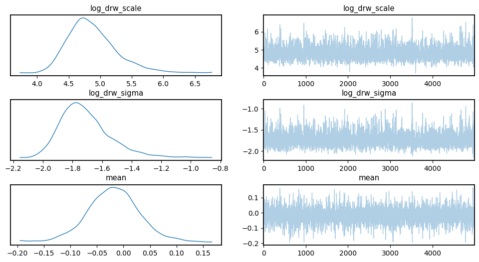
3.2 Visualize Chains, Posterior Distributions#

[13]:

az.plot_trace(
    data,
    var_names=["log_drw_scale", "log_drw_sigma", "mean"],
)
plt.subplots_adjust(hspace=0.4)

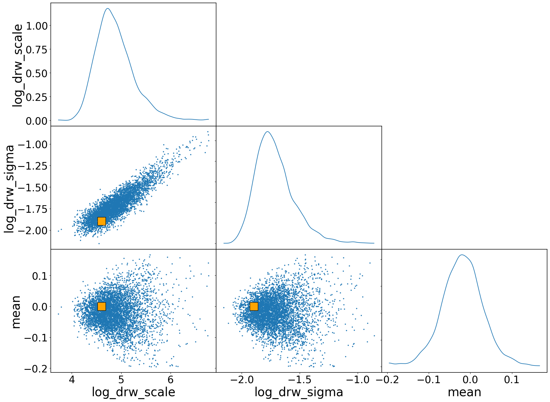
[14]:

az.plot_pair(
    data,
    var_names=["log_drw_scale", "log_drw_sigma", "mean"],
    reference_values={
        "log_drw_scale": np.log(drw_scale),
        "log_drw_sigma": np.log(drw_sigma),
        "mean": 0.0,
    },
    reference_values_kwargs={"color": "orange", "markersize": 20, "marker": "s"},
    kind="scatter",
    marginals=True,
    textsize=25,
)
plt.subplots_adjust(hspace=0.0, wspace=0.0)

4. Second-order Statistics#

EzTaoX provides a unified class (extaox.kernel_stat2.gpStat2) for generating the second-order statistic functions (ACF, SF, and PSD) of any supported kernels. All you need to do is initialize a gpStat2 instance with your desired kernel

[15]:

from eztaox.kernel_stat2 import gpStat2

ts = np.logspace(0, 4)
fs = np.logspace(-4, 0)

[16]:

# get MCMC samples
flatPost = data.posterior.stack(sample=["chain", "draw"])
log_drw_draws = flatPost["log_kernel_param"].values.T

[17]:

# create second-order stat object
drw_k = Exp(scale=drw_scale, sigma=drw_sigma)
gpStat2_drw = gpStat2(drw_k)

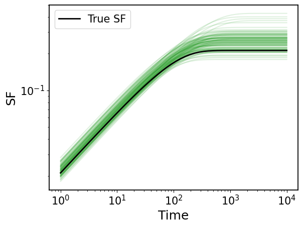
4.1 Structure Function#

[18]:

# compute sf for MCMC draws
mcmc_sf = jax.vmap(gpStat2_drw.sf, in_axes=(None, 0))(ts, jnp.exp(log_drw_draws))

[19]:

## plot
# ture SF
plt.loglog(ts, gpStat2_drw.sf(ts), c="k", label="True SF", zorder=100, lw=2)
plt.legend(fontsize=15)
# MCMC SFs
for sf in mcmc_sf[::50]:
    plt.loglog(ts, sf, c="tab:green", alpha=0.15)

plt.xlabel("Time")
plt.ylabel("SF")

[19]:

Text(0, 0.5, 'SF')

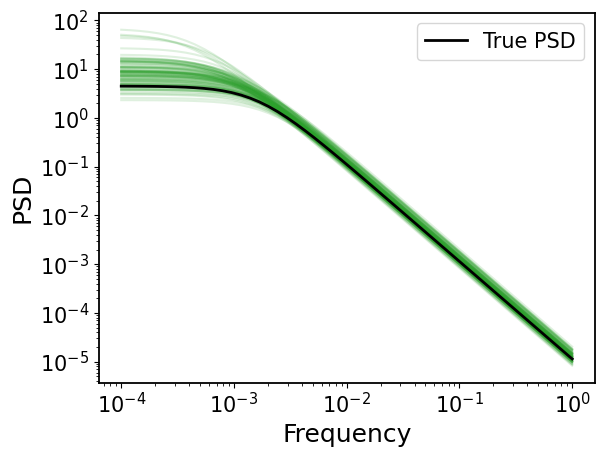
4.2 Power Spectral Density (PSD)#

[20]:

# compute sf for MCMC draws
mcmc_psd = jax.vmap(gpStat2_drw.psd, in_axes=(None, 0))(fs, jnp.exp(log_drw_draws))

[21]:

## plot
# ture PSD
plt.loglog(fs, gpStat2_drw.psd(fs), c="k", label="True PSD", zorder=100, lw=2)
plt.legend(fontsize=15)

# MCMC PSDs
for psd in mcmc_psd[::50]:
    plt.loglog(fs, psd, c="tab:green", alpha=0.15)

plt.xlabel("Frequency")
plt.ylabel("PSD")

[21]:

Text(0, 0.5, 'PSD')