[1]:
import matplotlib as mpl
import matplotlib.pyplot as plt
import numpy as np

mpl.rcParams.update(
    {
        "text.usetex": False,
        "axes.labelsize": 18,
        "xtick.labelsize": 15,
        "ytick.labelsize": 15,
        "figure.constrained_layout.wspace": 0,
        "figure.constrained_layout.hspace": 0,
        "figure.constrained_layout.h_pad": 0,
        "figure.constrained_layout.w_pad": 0,
        "axes.linewidth": 1.3,
    }
)

import jax
import jax.numpy as jnp

# you should always set this
jax.config.update("jax_enable_x64", True)
Transfer Functions and Convolved Kernels#
In astrophysics, many observed signals are not direct realizations of a simple stochastic process — they are responses to an underlying (latent) driving process. For example, in reverberation mapping of active galactic nuclei (AGN), the accretion disk continuum emission drives variability in the broad emission-line region (BLR). The BLR responds to the continuum with a characteristic time delay and smoothing, described by a transfer function \(\Psi(\Delta t)\).
Mathematically, if the latent (driving) process is \(X(t)\), the observed (response) process is:
The key property that makes this tractable is the Wiener–Khinchin theorem: if \(X(t)\) is a stationary GP with power spectral density \(S_X(f)\), then \(Y(t)\) is also a stationary GP with PSD
where \(\hat{\Psi}\) is the Fourier transform of the transfer function. Equivalently, \(Y\) has a convolved kernel:
EzTaoX implements this via ConvolvedKernel, which takes any quasisep kernel and a transfer function, computes the convolved kernel via FFT, and exposes it as a standard GP kernel. This means you can use the convolved kernel directly in GP inference — no need to explicitly model the latent process.
In this notebook we demonstrate:
Compare two ways to simulate \(Y(t)\):
Explicit convolution: simulate the latent \(X(t)\) and convolve with \(\Psi\). This method requires simmulating the lattent process and performing the convolution for each realization.
Direct GP draw: simulate directly from the GP with
ConvolvedKernel.
How the structure function (SF) validates that both approaches produce statistically equivalent processes.
1. Setup: Parameters and Transfer Function#
We model the latent driving process as a Damped Random Walk (DRW), i.e., an Ornstein–Uhlenbeck process with the exponential kernel
The transfer function is a symmetric Gaussian centred at zero:
normalized so that \(\int \Psi(s)\,ds = 1\). For a causal (one-sided) echo model, see CausalGaussianTransferFunction or CausalExponentialTransferFunction.
We choose \(\tau = 100\) (DRW damping timescale), \(\sigma = 1\) (amplitude), and \(w = 20\) (transfer function width), so the echo smoothing is noticeably shorter than the variability timescale.
[2]:
from tinygp.kernels import Exp as ExpDirect

from eztaox.kernel_stat2 import gpStat2
from eztaox.kernels import quasisep
from eztaox.kernels.transfer_function import (
    ConvolvedKernel,
    GaussianTransferFunction,
)
from eztaox.simulator import UniVarSim

# ── parameters ──────────────────────────────────────────────────────────────
tau = 100.0  # DRW damping timescale
sigma = 1.0  # DRW amplitude
psi_width = 20.0  # Gaussian transfer function width
rng_seed = 0

# ── kernels and transfer function ────────────────────────────────────────────
transfer_function = GaussianTransferFunction(width=psi_width)
base_kernel = quasisep.Exp(scale=tau, sigma=sigma)
convolved_kernel = ConvolvedKernel(base_kernel, transfer_function, n_grid=2000)
2. Approach A — Explicit Convolution#
Here we:
Simulate the latent DRW light curve \(X(t)\) on a dense, evenly-spaced grid.
Build the transfer function kernel \(\Psi(\Delta t)\) on the same grid (centred at zero, so it covers both positive and negative lags).
Convolve \(X\) with \(\Psi\) via FFT to obtain the expected response \(Y_{\mathrm{conv}}(t)\).
The result \(Y_{\mathrm{conv}}\) is a single specific realization of the response process, derived deterministically from \(X\).
[3]:
n = 1000
t = jnp.linspace(0.0, 1000.0, n)
dt = float(t[1] - t[0])

n_realizations = 10

# ── build the latent simulator once ─────────────────────────────────────────
sim_latent = UniVarSim(
    ExpDirect(scale=tau),
    1.0,
    float(t[-1]),
    init_params={"log_kernel_param": jnp.array([jnp.log(tau)])},
    zero_mean=True,
)

# ── build Ψ on a symmetric grid (same for all realizations) ─────────────────
t_kernel = jnp.r_[-t[::-1][1:], t]  # length 2n-1, zero at centre
kernel_vals = jax.vmap(transfer_function.evaluate)(jnp.zeros_like(t_kernel), t_kernel)

# ── simulate n_realizations pairs (latent + convolved) ──────────────────────
lcs_latent = []
lcs_expected = []
for seed in range(n_realizations):
    _, lc_lat = sim_latent.fixed_input_fast(t, jax.random.PRNGKey(seed))
    lc_exp = jax.scipy.signal.fftconvolve(lc_lat, kernel_vals, mode="same") * dt
    lcs_latent.append(lc_lat)
    lcs_expected.append(lc_exp)
3. Approach B — Direct GP Draw from the Convolved Kernel#
Instead of simulating a latent process and convolving, we can draw directly from a GP whose kernel is \(k_Y\) — computed by ConvolvedKernel via the Wiener–Khinchin relation in Fourier space.
The two approaches use different random seeds, so the resulting light curves can only be compared statistically, not realization-by-realization.
[4]:
sim_convolved = UniVarSim(
    convolved_kernel,
    1.0,
    float(t[-1]),
    init_params={
        "log_kernel_param": jnp.array(
            [jnp.log(tau), jnp.log(sigma), jnp.log(psi_width)]
        )
    },
    zero_mean=True,
)

# use seeds n_realizations … 2*n_realizations-1 to keep all 20 distinct
lcs_actual = []
for seed in range(n_realizations, 2 * n_realizations):
    _, lc_act = sim_convolved.fixed_input_fast(t, jax.random.PRNGKey(seed))
    lcs_actual.append(lc_act)
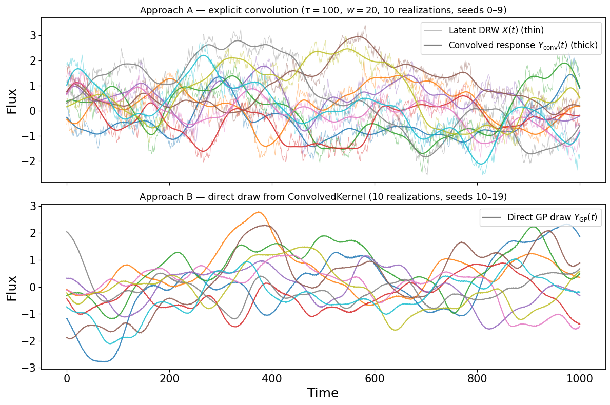
4. Light Curve Comparison#
We draw 10 independent realizations per approach and show them on two separate panels.
Top panel — each color is one simulation run: the thin semi-transparent line is the latent DRW \(X(t)\), and the thick line is its convolved response \(Y_{\mathrm{conv}}(t) = (\Psi * X)(t)\). Because the response is derived from that specific latent draw, it tracks its broad features.
Bottom panel — 10 independent GP draws directly from ConvolvedKernel, one color each. These use completely different random seeds; they are unrelated to the top-panel realizations.
Visually, both panels should show the same spread and smoothness — the same statistical ensemble — even though no individual pair matches. That is the whole point: ConvolvedKernel encodes the correct statistics without needing to simulate the latent process explicitly.
[5]:
colors = [mpl.colormaps["tab10"](i) for i in range(n_realizations)]

fig, axes = plt.subplots(2, 1, figsize=(12, 8), sharex=True)

# ── top panel: latent (thin) + convolved (thick), same color per run ─────────
ax = axes[0]
for i, (lc_lat, lc_exp) in enumerate(zip(lcs_latent, lcs_expected)):
    ax.plot(np.asarray(t), np.asarray(lc_lat), color=colors[i], lw=0.8, alpha=0.4)
    ax.plot(np.asarray(t), np.asarray(lc_exp), color=colors[i], lw=1.6, alpha=0.85)
# legend proxies
ax.plot([], [], color="gray", lw=0.8, alpha=0.5, label="Latent DRW $X(t)$ (thin)")
ax.plot(
    [], [], color="gray", lw=1.6, label=r"Convolved response $Y_{\rm conv}(t)$ (thick)"
)
ax.set_ylabel("Flux")
ax.legend(fontsize=12, loc="upper right")
ax.set_title(
    r"Approach A — explicit convolution ($\tau={tau},\;w={w}$, 10 realizations, seeds 0–9)".format(
        tau=int(tau), w=int(psi_width)
    ),
    fontsize=13,
)

# ── bottom panel: direct GP draws ────────────────────────────────────────────
ax = axes[1]
for i, lc_act in enumerate(lcs_actual):
    ax.plot(np.asarray(t), np.asarray(lc_act), color=colors[i], lw=1.6, alpha=0.85)
ax.plot([], [], color="gray", lw=1.6, label=r"Direct GP draw $Y_{\rm GP}(t)$")
ax.set_xlabel("Time")
ax.set_ylabel("Flux")
ax.legend(fontsize=12, loc="upper right")
ax.set_title(
    "Approach B — direct draw from ConvolvedKernel (10 realizations, seeds 10–19)",
    fontsize=13,
)

fig.tight_layout()
plt.show()
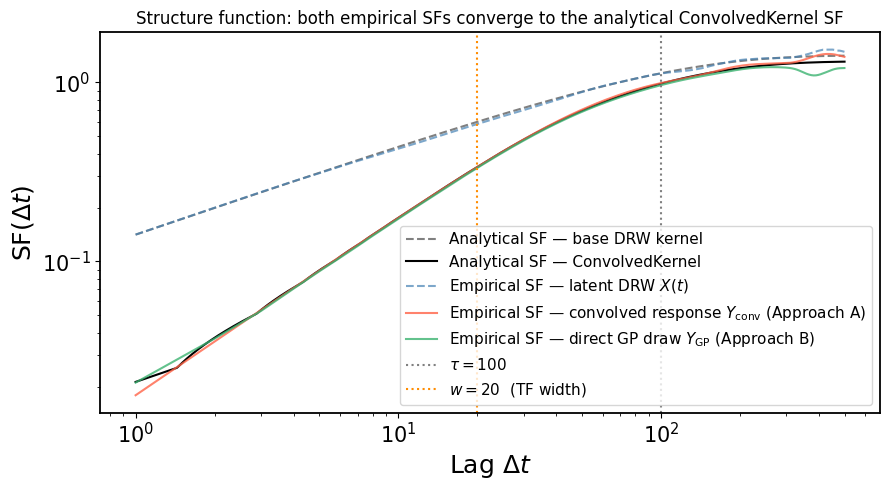
5. Structure Function Comparison#
The structure function (SF) measures the typical variability amplitude as a function of time lag:
For a stationary GP with kernel \(k\) and variance \(\sigma^2 = k(0)\), the theoretical SF is
We compare:
Empirical SF of the latent process \(X(t)\) — the DRW driver before convolution.
Empirical SF of \(Y_{\mathrm{conv}}\) — the explicitly convolved response (Approach A).
Empirical SF of \(Y_{\mathrm{GP}}\) — the direct GP draw from
ConvolvedKernel(Approach B).Analytical SF from ``ConvolvedKernel`` — computed via
gpStat2, using the exact convolved kernel.Analytical SF of the base DRW kernel — for reference.
If everything is consistent, the two empirical SFs of the response (Approach A and B) should both agree with the analytical SF of the convolved kernel, while both sitting below the raw DRW SF at short lags (the transfer function smooths out short-timescale fluctuations).
[6]:
# ── empirical SF helper ───────────────────────────────────────────────────────
def empirical_sf(lc, ks):
    """Compute empirical structure function at integer lag indices ks."""
    return jnp.array([jnp.sqrt(jnp.mean((lc[k:] - lc[:-k]) ** 2)) for k in ks])


# shared max lag for both empirical and analytical curves
max_lag = float(t[-1]) / 2

lag_indices = jnp.unique(jnp.geomspace(1, round(max_lag / dt), 300).round().astype(int))
lags_empirical = np.asarray(lag_indices) * dt

# use all realizations and average the SFs for a more robust estimate
sf_latent = np.mean([empirical_sf(lc, lag_indices) for lc in lcs_latent], axis=0)
sf_expected = np.mean([empirical_sf(lc, lag_indices) for lc in lcs_expected], axis=0)
sf_actual = np.mean([empirical_sf(lc, lag_indices) for lc in lcs_actual], axis=0)

# ── analytical SFs ───────────────────────────────────────────────────────────
lags_theory = jnp.geomspace(dt, max_lag, 500)
sf_theory_convolved = gpStat2(convolved_kernel).sf(lags_theory)
sf_theory_base = gpStat2(base_kernel).sf(lags_theory)
[7]:
fig, ax = plt.subplots(figsize=(9, 5))

# ── analytical curves first (drawn underneath empirical) ─────────────────────
ax.loglog(
    np.asarray(lags_theory),
    np.asarray(sf_theory_base),
    lw=1.5,
    color="gray",
    linestyle="--",
    label="Analytical SF — base DRW kernel",
)
ax.loglog(
    np.asarray(lags_theory),
    np.asarray(sf_theory_convolved),
    lw=1.5,
    color="black",
    label="Analytical SF — ConvolvedKernel",
)

# ── empirical curves on top ───────────────────────────────────────────────────
ax.loglog(
    lags_empirical,
    np.asarray(sf_latent),
    linestyle="--",
    alpha=0.7,
    color="steelblue",
    label=r"Empirical SF — latent DRW $X(t)$",
)
ax.loglog(
    lags_empirical,
    np.asarray(sf_expected),
    alpha=0.8,
    color="tomato",
    label=r"Empirical SF — convolved response $Y_{\rm conv}$ (Approach A)",
)
ax.loglog(
    lags_empirical,
    np.asarray(sf_actual),
    alpha=0.8,
    color="mediumseagreen",
    label=r"Empirical SF — direct GP draw $Y_{\rm GP}$ (Approach B)",
)

# reference lines
ax.axvline(tau, color="gray", linestyle=":", lw=1.5, label=rf"$\tau = {tau:.0f}$")
ax.axvline(
    psi_width,
    color="darkorange",
    linestyle=":",
    lw=1.5,
    label=rf"$w = {psi_width:.0f}$  (TF width)",
)

ax.set_xlabel("Lag $\\Delta t$")
ax.set_ylabel("SF$(\\Delta t)$")
ax.set_title(
    "Structure function: both empirical SFs converge to the analytical ConvolvedKernel SF",
    fontsize=12,
)
ax.legend(fontsize=11, loc="best")
fig.tight_layout()
plt.show()
6. Interpretation#
The plot above illustrates several key points:
Short lags (\(\Delta t \ll w\)): The transfer function smooths out fluctuations faster than \(w\), so the convolved SF rises more slowly than the raw DRW SF. Below the transfer function width (orange dotted line), the response process appears nearly constant — it cannot resolve structure shorter than the echo timescale.
Long lags (\(\Delta t \gg \tau\)): Both the latent and convolved processes saturate to their asymptotic variance. Because the transfer function is normalized to unity, the long-lag SF of the response equals that of the driver.
Agreement between Approach A and Approach B: The empirical SFs of lc_expected (red) and lc_actual (green) both track the analytical ConvolvedKernel SF (black solid line). The mild scatter is due to finite sample size and is expected. This validates that ConvolvedKernel correctly encodes the statistics of the convolved process — you can use it directly in GP inference without explicitly simulating the latent process.
Available transfer functions#
Class |
Shape |
Causal? |
|---|---|---|
|
Symmetric Gaussian |
No |
|
Symmetric two-sided exponential |
No |
|
One-sided Gaussian (\(\Delta t \ge 0\)) |
Yes |
|
One-sided exponential (\(\Delta t \ge\) shift) |
Yes |
All transfer functions satisfy \(\int \Psi(s)\,ds = 1\), ensuring the response process has the same asymptotic variance as the driver. Currently implemented transfer functions are not supposed to be used for real reverberation mapping simulations, but they demonstrate how to build custom transfer functions. For more realistic BLR echo models, you can implement your own TransferFunction subclass by defining the evaluate method, which should return \(\Psi(\Delta t)\) for given lag
values.