import numpy as np
import matplotlib.pyplot as plt
import matplotlib as mpl
import warnings

warnings.filterwarnings("ignore", category=RuntimeWarning)

mpl.rcParams.update(
    {
        "text.usetex": False,
        "axes.labelsize": 20,
        "figure.labelsize": 18,
        "xtick.labelsize": 16,
        "ytick.labelsize": 16,
        "figure.constrained_layout.wspace": 0,
        "figure.constrained_layout.hspace": 0,
        "figure.constrained_layout.h_pad": 0,
        "figure.constrained_layout.w_pad": 0,
        "axes.linewidth": 1.2,
    }
)

import jax
import jax.numpy as jnp

# you should always set this
jax.config.update("jax_enable_x64", True)

Simulating Multi-band Light Curves

This notebook demonstrates how to use MultiVarSim to simulate multi-band light curves with EzTaoX. We assume a damped random walk (DRW) latent kernel and show how to draw full light curves, randomly sampled observations, and observations on a user-provided cadence.

from eztaox.kernels.quasisep import Exp
from eztaox.simulator import MultiVarSim
from eztaox.ts_utils import add_noise, formatlc

1. Initialize a multiband simulator

The multiband simulator assumes that all bands share the same latent GP kernel, while each observed band can have its own amplitude, mean, and lag. In the default EzTaoX convention, the band with index 0 is the reference band, so log_amp_scale and lag only need M-1 entries for the remaining bands.

band_order = {"g": 0, "r": 1, "i": 2}
band_names = tuple(band_order.keys())
band_colors = {"g": "tab:green", "r": "tab:red", "i": "tab:orange"}

# latent DRW parameters
drw_scale = 120.0
drw_sigma = 0.18

# observed-band amplitudes, means, and lags
amp_scale = {"g": 1, "r": 0.7, "i": 0.5}
mean = {"g": 0.0, "r": 0.0, "i": 0.0}
lag = {"g": 0.0, "r": 4.0, "i": 9.0}

sim_params = {
    "log_kernel_param": jnp.log(jnp.asarray([drw_scale, drw_sigma])),
    "log_amp_scale": jnp.log(jnp.asarray([amp_scale["r"], amp_scale["i"]])),
    "mean": jnp.asarray([mean[band] for band in band_names]),
    "lag": jnp.asarray([lag["r"], lag["i"]]),
}

min_dt, max_dt = 1.0, 3650.0
kernel = Exp(scale=drw_scale, sigma=drw_sigma)

simulator = MultiVarSim(
    kernel,
    min_dt,
    max_dt,
    n_band=len(band_order),
    init_params=sim_params,
    zero_mean=False,
    has_lag=True,
)
simulator

MultiVarSim(
  base_kernel_def=<jax._src.util.HashablePartial object at 0x751538579a50>,
  multiband_kernel=<class 'eztaox.kernels.quasisep.MultibandLowRank'>,
  X=(f64[10953], i64[10953]),
  init_params={
    'log_kernel_param':
    f64[2],
    'log_amp_scale':
    f64[2],
    'mean':
    f64[3],
    'lag':
    f64[2]
  },
  n_band=3,
  mean_func=None,
  amp_scale_func=None,
  lag_func=None,
  zero_mean=False,
  has_lag=True
)

def split_by_band(X, y, band_order):
    inverse_band_order = {idx: band for band, idx in band_order.items()}
    ts, ys = {}, {}

    for idx, band in inverse_band_order.items():
        mask = X[1] == idx
        order = jnp.argsort(X[0][mask])
        ts[band] = X[0][mask][order]
        ys[band] = y[mask][order]

    return ts, ys

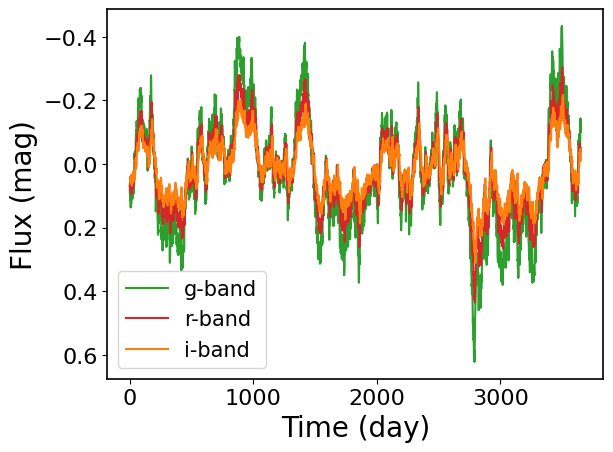
2. Simulate a full multi-band light curve

The full method returns a uniformly sampled realization of the multi-band GP on the simulator grid. This is useful when you want to inspect the latent variability pattern before imposing an observing cadence.

full_X, full_y = simulator.full(jax.random.PRNGKey(0))
full_ts, full_ys = split_by_band(full_X, full_y, band_order)

for band in band_names:
    plt.plot(full_ts[band], full_ys[band], c=band_colors[band], label=f"{band}-band")

plt.gca().invert_yaxis()
plt.xlabel("Time (day)")
plt.ylabel("Flux (mag)")
plt.legend(fontsize=15)

<matplotlib.legend.Legend at 0x75153836ccd0>

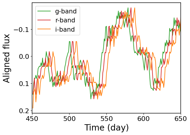
2.1 Zoom in to highlight the inter-band delays

The full realization already includes the lags, but they are easier to see over a shorter time range. In the plot below, we zoom in on one section of the simulated light curve and remove the band-dependent mean and amplitude scaling so the same latent variability pattern can be compared directly across bands.

zoom_min, zoom_max = 450.0, 650.0

for band in band_names:
    mask = (full_ts[band] >= zoom_min) & (full_ts[band] <= zoom_max)
    aligned_flux = (full_ys[band][mask] - mean[band]) / amp_scale[band]
    plt.plot(
        full_ts[band][mask],
        aligned_flux,
        c=band_colors[band],
        label=f"{band}-band",
    )

plt.gca().invert_yaxis()
plt.xlabel("Time (day)")
plt.ylabel("Aligned flux")
plt.xlim(zoom_min, zoom_max)
plt.legend(fontsize=15)

<matplotlib.legend.Legend at 0x751529637390>

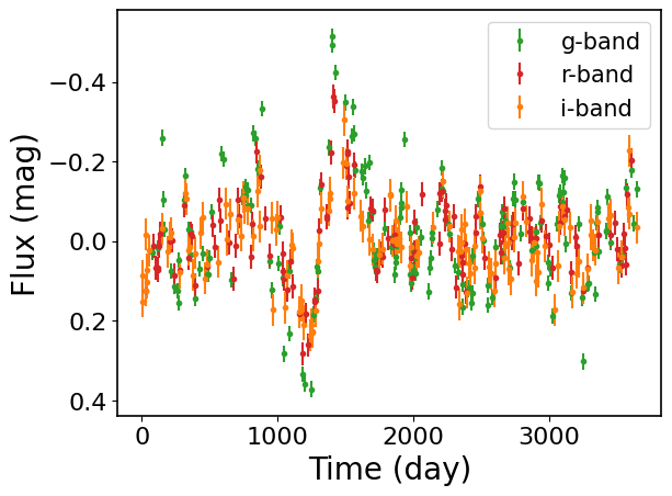
3. Simulate randomly sampled observations

The random method first generates a full multi-band realization and then draws a random subset of observations from it. This is a convenient way to make a mock light curve with irregular sampling. Here we also add band-dependent photometric noise.

random_X, random_y = simulator.random(
    450,
    jax.random.PRNGKey(1),
    jax.random.PRNGKey(2),
)
random_ts, random_ys = split_by_band(random_X, random_y, band_order)

noise_level = {"g": 0.02, "r": 0.03, "i": 0.04}
random_yerr, random_y_noisy = {}, {}

for i, band in enumerate(band_names):
    random_yerr[band] = jnp.ones_like(random_ys[band]) * noise_level[band]
    random_y_noisy[band] = add_noise(
        random_ys[band], random_yerr[band], jax.random.PRNGKey(10 + i)
    )

for band in band_names:
    plt.errorbar(
        random_ts[band],
        random_y_noisy[band],
        random_yerr[band],
        fmt=".",
        c=band_colors[band],
        label=f"{band}-band",
    )

plt.gca().invert_yaxis()
plt.xlabel("Time (day)")
plt.ylabel("Flux (mag)")
plt.legend(fontsize=15)

<matplotlib.legend.Legend at 0x7515285c3f90>

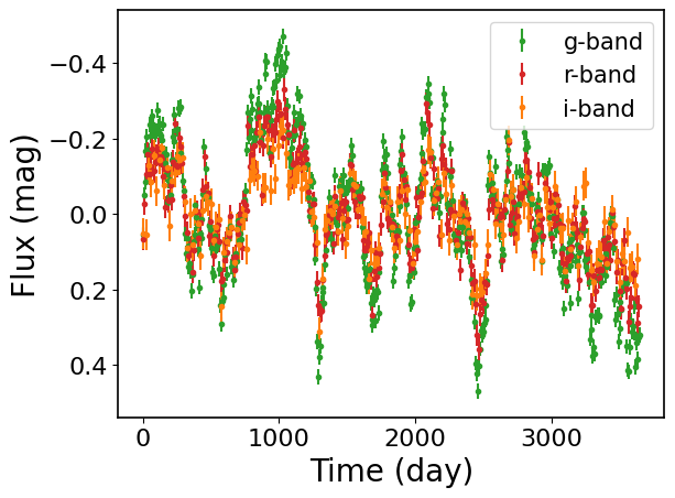
4. Simulate observations on a user-provided cadence

If you already know the observing times in each band, you can build the input coordinates explicitly and simulate the GP on that cadence. The helper function formatlc is convenient for turning per-band dictionaries into the (time, band) format expected by EzTaoX. In this example, we use fixed_input_fast, which evaluates the GP directly on the requested cadence.

cadence_ts = {
    "g": jnp.arange(0.0, 3650.0, 7.0),
    "r": jnp.arange(2.0, 3650.0, 11.0),
    "i": jnp.arange(5.0, 3650.0, 19.0),
}

dummy_y = {band: jnp.zeros_like(ts) for band, ts in cadence_ts.items()}
dummy_yerr = {band: jnp.ones_like(ts) for band, ts in cadence_ts.items()}
input_X, _, _ = formatlc(cadence_ts, dummy_y, dummy_yerr, band_order)
input_X

(Array([   0.,    7.,   14., ..., 3596., 3615., 3634.], dtype=float64),
 Array([0, 0, 0, ..., 2, 2, 2], dtype=int64))

cadence_X, cadence_y = simulator.fixed_input_fast(input_X, jax.random.PRNGKey(3))
cadence_split_ts, cadence_split_ys = split_by_band(cadence_X, cadence_y, band_order)

cadence_yerr, cadence_y_noisy = {}, {}

for i, band in enumerate(band_names):
    cadence_yerr[band] = jnp.ones_like(cadence_split_ys[band]) * noise_level[band]
    cadence_y_noisy[band] = add_noise(
        cadence_split_ys[band], cadence_yerr[band], jax.random.PRNGKey(20 + i)
    )

for band in band_names:
    plt.errorbar(
        cadence_split_ts[band],
        cadence_y_noisy[band],
        cadence_yerr[band],
        fmt=".",
        c=band_colors[band],
        label=f"{band}-band",
    )

plt.gca().invert_yaxis()
plt.xlabel("Time (day)")
plt.ylabel("Flux (mag)")
plt.legend(fontsize=15)

<matplotlib.legend.Legend at 0x75151f6af390>